
This summer the website of The Economist Magazine published Height of Romance: The deceptive rise of the “short king”, about the challenges of short men in the cohabitation and marriage market. That piece included a graphic that violated a cardinal rule for data representation: Be clear in the message you wish to convey. I decided to explore why the graphic confused me, and to fix its oversights with something I call a brownie chart.
Here is the data visualization, intended to show the many instances in survey data of heterosexual households where the man is more often taller than the woman than expected against a normal curve (i.e., a purely random distribution in the shape of a smoothly sloped hill, or “bell”):
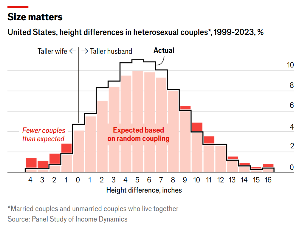
The graphic used data from the America’s Panel Study of Income Dynamics for 1999-2023, which interviews roughly 9,000 families every two years.
The intended conclusion was that opposite-sex couples are far more likely to set up a household where he is taller than her than randomness would predict. If you’re like me, you had to spend a long time staring at it to pick up that message. Forcing a reader to struggle is data visualization death.
I love The Economist, and even wrote as much recently on my personal blog, A love letter to shared facts and The Economist. I mentioned in that post the extreme rigor of their copy editing process, and found it significant that the article never made it to the print edition. My theory is the editor decided that the article itself was solid but this illustration was too vague to warrant putting ink to paper.
Wise move.
I get it: The data analyst and visualization designer would be understandably tempted to show a normal curve against the measured differences. But the result isn’t instantly convincing.
I set out to fix it by replacing the bars describing the curves in the chart with a personal favorite of mine, the tree map, augmented with a heat map color-coding. It’s a graphics combo platter I’ve proudly renamed the brownie chart. I call it that for two reasons:
- It looks like a pan of irregularly sliced brownies
- It follows the convention of other area charts named after sugary treats, the pie chart and the donut chart
I first wrote about this charting technique 16 years ago, in my marketing technology blog, Visualizing bounce rates using brownie charts. Cute name aside, the brownie chart — now old enough in the U.S. to get a driver’s license — does real work.
Before I built my response to the bar chart, I considered something the Economist data analyst did not. My approach took into account sample sizes. This eliminated our bias to assume charts based on small sample sizes are always reliable.
You may ask, Was that necessary? After all, we’re looking at a respected survey of 9,000 households. How could something of that size contain uncertainty?
Most of the graphic’s cohorts fail a confidence test
My first step was to determine actual sample sizes for each bar in the Economist chart, since each represents an inch of height difference. To do that I reduced the 9,000 households number by taking the 2020 U.S. Census Data’s percentage of households with married or unmarried heterosexual couples. That portion is between 27 and 28 percent of all households (I split the difference and used 27.5%).
That’s a 72.5% reduction in the data universe. Suddenly the air in the data is getting thin.
Applying the stated percentages, I could calculate each cohort’s sample size. I then applied the same rule we’re used to seeing in analyzing an A/B test. Testing and personalization of consumer data is where I earn my living. I analyzed each cohort as a binary test, applying a p-value test using the individual inch bar values to see if we can be confident that the data it reports for the cohort can be believed.
The color-coding of this data table shows the following three states:
- He is taller than her more than randomness would predict (Baby Blue)
- She is taller than him more than randomness would predict (Barbie Pink)
- The data is inconclusive because the p-value is greater than or equal to 0.05 (Grey).
Here is that table:
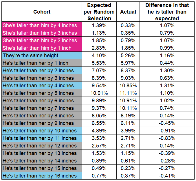
This high level of uncertainty is missing from the Economist chart. That’s a problem, because each bar in the chart is presumed trustworthy.
The size of rectangles in my brownie chart reflects the quantities of the expected outcome for that inch cohort. Similar to the way you’d read a pie chart or donut chart, the total area equals the entire universe of inch cohorts.
Household height selection trends as a brownie chart
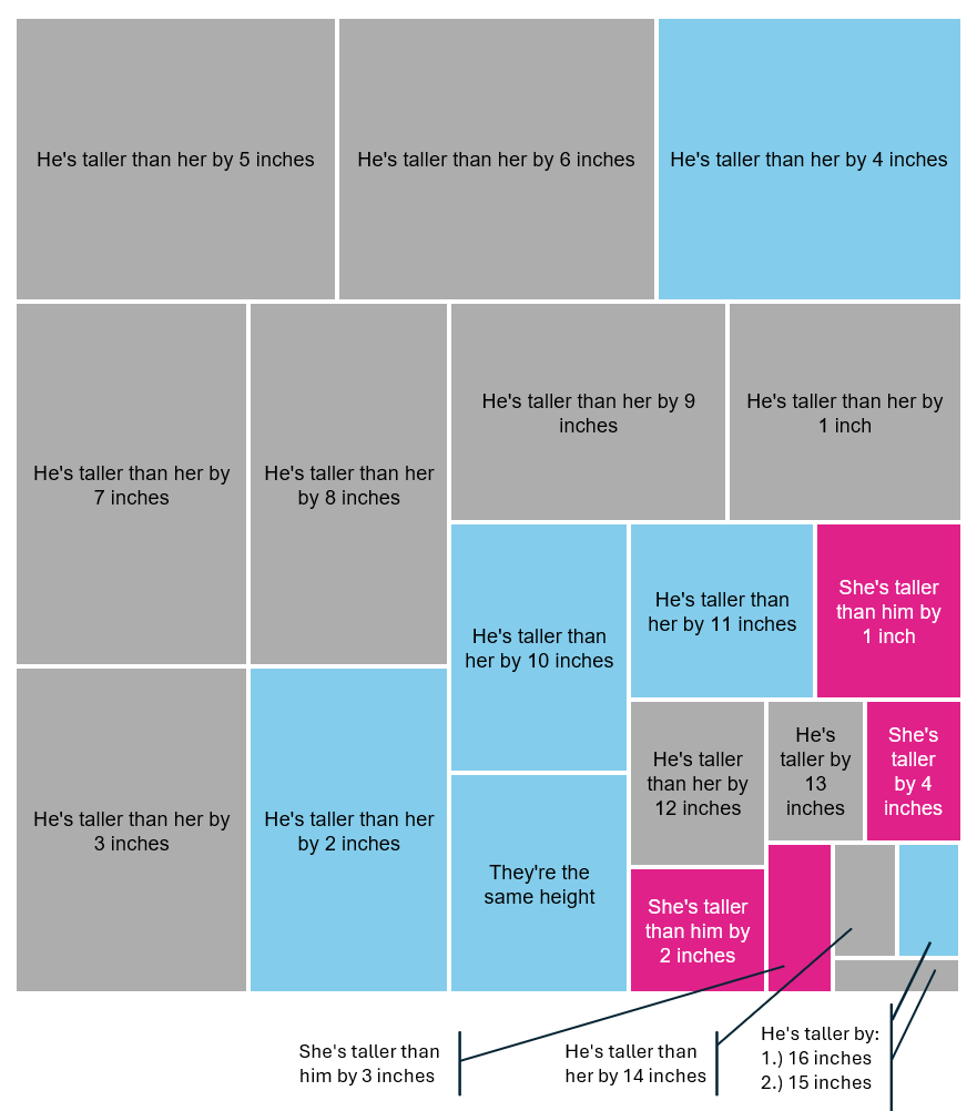
You may be surprised that some of the largest sample sizes show data that is not statistically valid. That’s because the difference between expected value and observed value was “too close to call,” even at that relatively large sample size.
The strength of a brownie chart is this interplay of size and color. It communicates clearly without losing sight of considerable statistical uncertainty. It’s obvious from the size of the grey rectangles that the largest area is of the sum of statistically uncertain cohorts (62.9% of the universe).
But the Economist was not wrong in how it interpreted the data set. For those that do show certainly, the point is quite clear, even at a glance:
There are far more men taller than the women in household pairings than one would expect based on randomness. The tendency toward taller women than their male mates, compared to what is randomly predicted, is only 7.2% of the universe. Yet the real versus predicted size for men being taller or the same height is 29.9% .
The brownie chart shows all of those comparisons instantly. Would my chart have made it into the print edition? Absolutely not.
No reader would find comfort in all this uncertainty. But life is full of the stuff, and since this survey is clearly the best source of data to investigate height biases in household pairings, one takes what one can get and seeks insights if possible.
And we do see trends that support the story.
My opinion is the editor should have ditched that bar chart altogether. The article alone made their point. From the data, they rolling up some of those cohorts to something statistically significant, and pointed out the following (the emphasis is mine):
The most common arrangement, accounting for around two-thirds of straight couples, is one in which the man is between two and eight inches taller than the woman (the average is 5.3 inches). Those in which the woman is taller account for just 3.3% of couples. … [Taking into account the baseline of random pairings], taller women would be expected in 7.2% of all couples. In other words, men are less than half as likely to partner with taller women than chance alone would predict.
In addition to their massive combined star power, it’s another reason why the marriage earlier this year of actors Tom Holland (5’ 8”) and Zendaya (5’ 10”) was so newsworthy.